The articles that will come in handy

Approximately 100,000 units of varying content come through our iFunny app daily, and every single one of them needs to be checked. We have already dealt with forbidden imagery by creating a classifier that automatically bans it. Next up — old memes, reuploads, and straight-up doubles that users try to sneak past the moderation.

To get rid of those, we have introduced a duplicate detection system. It had already gone through several iterations, but at some point, we realized it was impossible to put version-to-version improvements in proper perspective. And so we ventured into the Net, searching for books and articles that would allow us to examine currently existing approaches to duplicate detection and — most importantly — to their quality assessment. You can see what we’ve found below.

What is a duplicate of an image?

Defining “duplicate” is not as easy as it may seem. To begin with, there are several types of them, and let us introduce some crucial definitions for a better understanding.

The Hash Function converts an array of input data of arbitrary length into an output bit string of a specified size, and an algorithm performs it.

A perfect hash function requires certain conditions:

1. It must be deterministic — that is, the same message must result in the same hash value.

2. Its value must be rapidly calculated for each message.

3. Finding the message responsible for a particular hash value must be impossible.

4. It must be impossible for two different messages with the same hash value to exist.

5. A slight alteration to the message must change the hash so that the current and previous values do not seem to correlate.

Hash or hash sum is the hash function’s end result. The fourth condition dictates that hash is unique for each object, but in reality, it is not. Any value can be fed into the hash function, but there is a limited number of result variations. However, this number is so significant (2 to the power of 256 for a 256-bit hash) that detecting this error is highly improbable.

Now let us move on to duplicates. While they do not possess a mathematical definition, it is clear that elements matching each other in all criteria and parameters will be considered duplicates or copies of the same object.

The property given to hash can detect duplicates as elements that have coinciding hash sums. This means that objects that are similar to each other in any other way but have varying hash sums for different things are “near-duplicates.” ND in short.

There are two types of NDs:

• Identical near-duplicates (IND) are obtained from a single digital source through certain transformations (cropping, formatting, applying filters, etc.). For instance, an original photo and a processed Instagram photo.

Copyright

• Non-identical near-duplicates (NIND) are images with identical content (an object or a scene) but different lighting, movement, exposure, occlusion, and so forth. For instance, two photos from a set.

Copyright

What we were trying to find

Duplicates are not a widely discussed topic on the Net. Amounts of diverse content pumping through large platforms like Instagram, TikTok, or YouTube are so significant that they generally do not care about duplicates.

Our case is a little more complicated: we focus on humor, and the content’s uniqueness depends solely on the user’s sense of humor and wit. This is not a perfect system, as countless stock and old memes appear all over the place.

When it came to evaluating our duplicate detection algorithm, we identified two main questions.

— What memes are considered duplicates?

In the case of old memes, these are usually duplicates or near-duplicates — or, basically, re-uploads of the same picture. It gets more complicated with non-identical near-duplicates when the user preserves the original joke but visually refurbishes it by picking a new image or changing the font. How old memes affect the metrics (some users prefer form to content) is another matter to discuss. Especially given the range of possible transformations that allow creating identical near-duplicates gives a lot of space for creativity.

— Where do we get test selection for the assessment?

This issue is relatively resolved through an artificial dataset operating within the designated margin of acceptable IND transformations. It is also possible to mark existing objects or take a marked dataset.

So, during the initial analysis of useful materials, we narrowed everything down to two primary objectives:

1. Find existing datasets that contain duplicates.
2. Create a set of permitted IND transformations.

Once these problems are solved, you are faced with the issues of metrics and quality assessment performed on a test selection. We deemed this quite easy and did not pay much attention to it.

Article 1. Enhancing DPF for Near-Replica Image Recognition

Original: Enhancing DPF for near-replica image recognition

Authors: Yan Meng and E. Chang

Year of publication: 2003

This article will help you create your own IND dataset to test your duplicate detection algorithm. It describes in detail twelve types of image transformations that were included in the dataset. The number of images obtained as a result of the transformation is given in parentheses for each operation.

1. Coloring (3): tweaking the image’s RGB channels by 10%.

2. Contrast change (2): altering the difference in intensity between lighter and darker elements of the image.

3. Cropping (4): symmetrically removing the margins of each image by 5%, 10%, 20%, and 30%, then returning to the original size.

4. Spot number reduction (1).

5. Lowering of resolution (7): by 10%, 20%, 30%, 40%, 50%, 70%, and 90%.

6. Reflection (2): horizontal mirroring.

7. Format change (1): converting JPEG into GIF to compress the color space to a 256-color palette.

8. Framing (4): adding an external frame that takes up 10% of the image. Four images with a randomly colored frame.

9. Turns (4): 90, 180, and 270 degrees turn.

10. Scaling (6): increasing the image size by 2, 4, and 8 times, then returning to the original size and decreasing the image size by 2, 4, and 8 times, then returning to the original size.

11. Saturation change (5): changing saturation by 70%, 80%, 90%, 110%, and 120%.Intensity change (4): changing intensity by 80%, 90%, 110%, and 120%.

12. Intensity change (4): changing intensity by 80%, 90%, 110%, and 120%.

No dataset comes with the article, but clear instructions will make it rather easy to repeat the process on your own.

Article 2. Efficient Near-Duplicate Detection and Sub-Image Retrieval

Original: Efficient Near-duplicate Detection and Sub-image Retrieval-Intel Research

Authors: Yan Ke, Rahul Sukthankar, and Larry Huston

Year of publication: 2004

The fact that it’s Intel Research should’ve already drawn your attention. This material is rather old and a little out of date — still, Google Academia shows that it’s been cited in 635 works. The article references the methods of dataset creation outlined in the previous one — but with the addition of stricter transformation:

1. Cropping (3): by 50%, 70%, and 90%. Then returning to the original size.

2. Slice (3): applying affine transformation along the X-axis by 5, 10, and 15 degrees.

3. Intensity change (2): changing the image brightness by 50% and 150%.

4. Contrast change (2): increasing and decreasing the image contrast by three times.

These additional transformations are not particularly useful for us, as they are not very applicable to memes (especially the 50%+ cropping), but some readers may use that to increase their selection.

Intel Research defines near-duplicates as images changed by common transformations: change of contrast or saturation, scaling, cropping, etc. According to the article, the ND detection system should have the following:

1. Recall. Every database image that contains sub-images present in the query image must be found, even if the sub-images take up only a small part of the original.

2. Precision. If the database and query images do not share nested images, they should not be matched. This is important, as incorrect marking of images will take up the user’s time.

3. Efficiency. Image query should take as little time as possible in order for the system to scale to huge databases.

The authors state that most ND-detection systems use [content-based image retrieval (CBIR). This approach has two flaws:

1. CBIR calculates and stores global statistics for each image. This, according to the authors, deals damage to both recall (due to significant transformations affecting the calculated statistics) and precision (due to some statistics being resistant to geometric transformations that lead to numerous false-positive responses)

2. CBIR calculates local statistics (for example, by splitting images into smaller parts), causing a decrease in the threshold value for comparing small parts of the feature vector. This, in turn, makes the vectors less discernible.

Without examples, both these statements seem rather abstract. But, judging by the description, the method of comparing neural network embeddings can be classified as CBIR. On the other hand, the authors offer to identify and independently index a large number of local features, each being resistant to image transformations.

This approach would selectively identify local objects that match well rather than look for weak partial matches between complex global objects. A scheme like this would resist various distortions and cropping that destroy a significant part of the functions.

However, there is a drawback — one image can generate thousands of local objects, which will lead to one request requiring the system to search for each of them in a database comprising millions of objects. Since there are no exact matches between the objects, each individual query will become a similar query in a very multidimensional space. This approach is not mathematically practical and thus not very popular. Still, the article shows that these ideas can become the basis for a near-duplicate and sub-image detection system that will be accurate and scalable for extensive collections of images.

The method implies using more different local descriptors, combined detectors of points of interest, independent of scale and rotation, and geometric verification of the matched features. Instead of an approximate similarity search, locally sensitive hashing is used. It is an algorithm with provable performance limits (and thus increased precision). The last essential feature is creating off-line indexes optimized for disk access and searching for all local descriptor queries in one go. This allows to drastically increase the speed of ND detection.

Article 3. Near Duplicate Image Detection: min-Hash and tf-idf Weighting

Original: Near Duplicate Image Detection: min-Hash and tf-idf Weighting

Authors: Ondřej Chum, James Philbin, and Andrew Zisserman

Year of publication: 2008

The article suggests extracting features through scale-invariant feature transform (SIFT) and then, with min-hash, searching for the matches between objects.

The authors assess the accuracy of the algorithms using two datasets:

• TrecVid 2006–146,588 frames automatically selected from 165 hours of news footage (17.8 million frames, 127 GB, JPEG). Each frame has a resolution of 352 x 240 pixels and is of low quality. Apart from the 2006 database, data for each year from 2001 to 2021 can be found on the site.
• University of Kentucky database — 10,200 images in sets of 4 images per 1 object/scene.

The second dataset seems more suitable for numerical metrics calculation. They do that in the article, with the first one used for visual analysis. Sadly, we have yet been unable to find the Kentucky dataset.

Results from the article dedicated to this database:

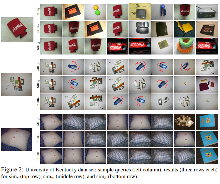
Nice idea, though — taking adjacent frames from a video and using them as non-identical near-duplicate images.

Article 4. Benchmarking Unsupervised Near-Duplicate Image Detection

Original: Benchmarking unsupervised near-duplicate image detection

Author: Lia Morra

Year of publication: 2019

A great and relatively fresh article compares ND detection approaches with various metrics and datasets. The authors consider convolutional neural networks useful for extracting the image feature vector and at that surpassing traditional methods.

Validation datasets

The authors use four datasets to compare the models’ results, three of which are in public access.

• CLAIMS — a private dataset (the way it was accessed is not disclosed). It was created for insurance purposes, containing photographs of interiors and exteriors of commercial and residential buildings. All in all, there are 201,961 images obtained from 22,327 applications.

• MFND (MirFlickr near-duplicate) — a set of found near-duplicates of the MIRFLICKR dataset. A total of 1,958 (2,407 pairs) INDs and 379 NIND clusters. The authors increased those numbers to 3,825 and 10,454, respectively; half of the work was done manually.

• California-ND — 701 real user photos from a private collection. These include a lot of complex NIND unchanged by artificial transformations.

To solve the problem of markup ambiguity, all images were marked up by ten people (including the author of the photo) on the following condition: “Should any two (or more) images appear to you similar in appearance or concept, label them as near-duplicates.”

About 245,350 possible unique combinations and 4,609 image pairs were designated as ND at least once. It is worth noting that opinions on the markup diverged in 82% of cases. Photo pairs formed 107 NIND clusters, each of them containing 6.55 images on average.

• Holidays — a popular dataset for solving the problem of object extraction. It comprises private holiday photos, with each image being hi-res with a large scene variability (nature, man-made objects, fire, etc.).

The images were grouped into 500 parallel image clusters, each representing a disparate scene or object. In total, there are 1,491 images in the set and approx. 2.98 images per cluster. In aggregate, 2,072 ND pairs mostly belong to the NIND type.

Comparison metrics

The choice of metrics for result validation is discussed separately. The authors maintain that most models are based on a controlled search for K-nearest neighbors, not implying the numerical values of metrics. And only some of them considered the issue of quantifying the level of detection of near-duplicates limited by a certain threshold.

• ROC analysis — calculates TPR and FPR for each threshold value and analyses the resulting graph. With regard to detecting ND, this metric was discussed in detail in this article.

• Hard negative mining — assumes that a real data set would have a volume of images (not related to ND/NIND) larger than that of ND. Assessing every pair is impossible.

Hard negative mining extracts a compact NIND set from a large image collection. It starts with a subset of randomly selected images from the query, based on the assumption that there are no NDs in the collection. Pairwise distance from all other images in the collection is calculated for every query, with selected the most complex (with the shortest distance) examples. The authors mention two possible scenarios for further quality assessment:

— Selecting the nearest neighbors for each query

— Getting K-nearest neighbors for all queries, sorting them, then selecting the most complex pairs

You can learn more about this method here.

• Area under the ROC curve (ROC-AUC) — builds a ROC curve from the first method and calculates the area beneath it. A non-decreasing function where TPR=1, FPR=0 is the best scenario. Therefore, the closer the curve comes to the point (1,0), the larger the area under it and the better the model itself.

Compared models

• GIST — a biology-inspired function. It imitates human visual perception to gain approximate but brief context data. The input image passes through the following stages:

— Decomposition into N blocks with a spatial pyramid

— Filtering with multiple Gabor filters

— Summation with an object extractor that defines the “essence” of the image by capturing its reflections, rotations, changes in scale and lighting

Sadly, the authors provide no further information on the topic. To fully comprehend it, read this.

The authors also experimented with perceptive hashing, but the results were so bad they did not make it into the article.

• SPoC (Sum-Pooled Convolutional). Here, the features are extracted from the top of the pre-trained neural network’s convolution layer, with the length of the feature vector being proportional to the depth of the network.

The best results were obtained through feature extraction done after the ReLU activation. PCA compression was applied to the vectors and L2 normalization, which reduces the length of the vectors to one. VGG and ResNet variations were used as the architecture. You can read more about the subject here.

• R-Mac (maximum regional activation of convolutions) creates compact object vectors by encoding several image regions in one go.

First, it establishes subdomains using a fixed grid in the range of gradually decreasing scales from 1 to L. Then, max-pooling is applied to extract objects from each separate region. Each spatial object vector of the region is subject to further PCA and L2 processing and normalization. Finally, regional object vectors are combined to create a single image vector, which is then again normalized with L2.

• Deep Retrieval uses a Siamese network with a triplet loss ranking function applied during the learning process. This way, the network learns to place similar objects closer and dissimilar ones further in the feature space.

Let Iq be a query image with a descriptor q, I+ — a relevant image with a descriptor d+, and I- — an irrelevant image with a descriptor d-. The rank triplet loss is defined as

where “m” is a scalar controlling the indentation amount.

To test the network, a feature vector obtained from the last convolutional layer is used, with layers aggregating through sum-pooling and normalization.

The architecture includes an additional proposal network similar to the R-Mac network. This means that functions are calculated for several potential areas of interest, not for the entire image. This network was previously trained on a dataset of control points.

The Deep Retrieval method is very similar to the method using SimCLR for duplicate detection. We applied this method to our database, but that is a whole other story.

In conclusion

We had to rigorously hound half of the Net, seeking the necessary materials, but the results were worth it. Now we have a clear understanding of existing same types and their features and — most importantly — of where to go next.

We’ve collected four datasets with different conditions and formulated a set of requirements for creating identical artificial NDs. And thus, our initial task is accomplished. We hope that you will find this helpful material too.